Output BOLD Image Data Analysis

Once the GLM estimation has finished, you are ready to view the resulting statistical output maps. Given that the contrasts have already been specified in the design file, the results can be displayed as overlays either on a structural volume or on a single volume from the BOLD image time-series, which is described below under displaying statistical maps on an image volume. Then you should select an appropriate threshold, described below in threshold maps.

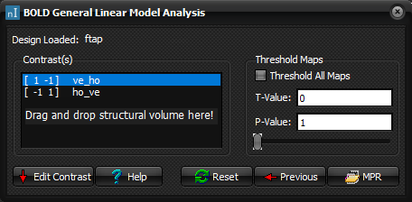
Please note that the BOLD image time series and structural volume should be from the same session. Otherwise, it will be problematic to display the generated statistical maps as overlays on the structural volume.

Contrast(s) list box

This is where the various specified contrasts are listed. The contrasts are needed to generate statistical output maps of the BOLD GLM analysis, using a T-test.

Note that if no contrasts are listed in the box, statistical output maps cannot be generated and displayed. Once valid contrasts are specified, the maps are generated and displayed as minimized windows. See displaying statistical maps on an image volume for information about how to visualize the maps as overlays. If these windows are closed, they can be reopened by clicking on the corresponding contrast in the list.

Note that a contrast can be deleted from the contrast(s) list box by right clicking on the contrast and choose Delete. See also edit contrast button for more information about modifying contrasts.

Displaying Statistical Maps on a structural volume

To display statistical output maps on an image volume as overlays, drag and drop the structural volume over the BOLD module window as indicated in figure above. The statistical output maps are then automatically added as overlays.

That is, follow this stepwise procedure:

1. Open the image volume where you would like to display the statistical output maps.

2. Click on this volume, using the left mouse button and hold it down.

3. Drag the volume, still pushing down the mouse button, into the square in the BOLD Module window, indicated with 'Drag and drop structural volume here!'.

4. Once the mouse pointer is positioned above the box, release the volume.

5. The statistical output maps are now automatically added to the dragged volume.

Note that if you would like to display the statistical output maps as overlays on single volume from the BOLD image time-series, set Scroll to Slice prior to drag and drop. See also sorting multi-dimensional datasets for more information.

Adding new contrasts or deleting or modifying an existing contrast might remove the displayed overlays. If this occurs, please perform the drag and drop operation again.

Display a Selection of Statistical Maps on an Image Volume

To display selection of statistical output maps as overlays, ensure that only the minimized windows of the statistical output maps that corresponds to the desired contrasts are displayed.

Modify Overlays

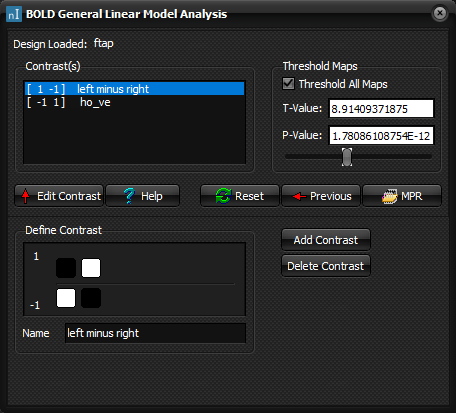
To modify or hide displayed overlay, right click on the image volume and choose Overlay->Modify... See overlay settings and modify image overlay for more information.

Threshold Maps

Once the statistical output maps, also called overlays, have been added to an image volume, you are ready to threshold the overlays. Overlays can be thresholded either individually, or they could all be given the same threshold value.

Threshold All Maps

Check for Threshold All Maps if you would like all overlays to have the same t-value threshold. Do not check mark if you would like to threshold each overlay individually. Then the overlay corresponding to the marked contrast in the Contrast(s) list box will be thresholded.

T-Value Threshold

Choose the minimum T-Value to display in the overlay. The corresponding P-Value will be estimated and updated automatically.

P-Value Threshold

Choose the P-value of the statistical output map. The corresponding T-Value will be estimated and updated automatically.

T-Value Slider

The T-Value slider allows you to interactively update the overlays while dragging the slider. The corresponding P- and T-Value will be updated automatically.

Other Options

Edit Contrast(s) button

This option allows you to add a new contrast, or delete an already specified contrast, after the GLM estimation has finished. An existing contrast can also be altered.

Add Contrast button

Adds a new, empty, contrast.

The contrast must be specified in define contrast prior to adding the corresponding statistical map as an overlay. It is not possible to generate a statistical map from an empty contrast.

Delete Contrast button

Delete the contrast which is marked in the contrast(s) list box. The corresponding statistical map will be deleted as well.

Define Contrast

This is where the contrast is specified. Click on the boxes to specify which regressor in the design matrix to weight against each other. In the above example, the resulting contrast will be [-1 1].

Note that the contrast, internally, will have an additional zero entry which is not displayed. It corresponds to the constant regressor in the design matrix, which is always added by the program.

Reset button

Deletes previous estimations. The loaded design file will be closed as well.
Note that previous preprocessing steps cannot be undone. To redo the preprocessing, please reload the original data.

MPR button

Display image volume, after drag and drop, using the multiplanar reconstruction tool (MPR).

Previous button

Go to the previous page.