Diffusion weighted analysis

The diffusion weighted imaging (DWI) analysis referrs to analysis of diffusion weighted MR images aquired using 1 or 3 diffusion encoding gradient directions. Prior to initiating this analysis module, it is of vital importance that the images are recognized as a 4-dimensional time-series (for multi-slice DWI images), and that the images are sorted according to image-number. This will be the case by default if the images were loaded either using the DICOM reader interface (see “ DICOM Reader ” ) or the DICOM server interface (see “ DICOM database ” ). 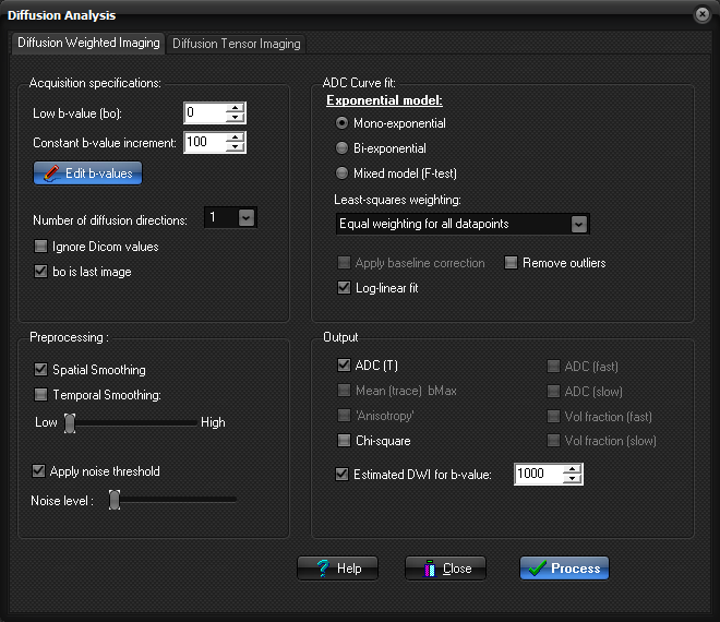Once loaded, the Diffusion Weighted Imaging tab can be displayed by selecting Diffusion Analysis (DWI) on the Modules menu.

Diffusion analysis settings.

nordicICE should be able to determine the acquisition specifications of the loaded dataset in most cases. If this fails, you need to know both the number of diffusion directions and corresponding b-values inherent in the dataset.

Acquisition specification:

Low b-value (b0): Specify the baseline (lowest) b-value. This is typically b0 but need not be so.
b-value increment: In case of more than two b-values and if the b-values have constant increment, then the b-value increment can be specified here.
Number of diffusion directions: This can be 1 or 3 directions.

Edit b-values: Used to specify the b-values of the diffusion gradients. Any number of b-values can be analyzed and if more than two b-values are used then a full non-linear exponential analysis is performed. The b-values should be entered in units of sec/mm^2.

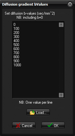
Example showing the setting of the b-values for analysis of DWI data holding multiple b-values. The b-values should be entered in units of sec/mm^2 and should include the b=0 value (if present in the input images).

NOTE: When performing the analysis, you may get a message informing that there are too few b-values in the list, and that some images are ignored. This can typically be the case if there are additional images to the DWI images in the loaded series, such as pre-calculated ADC-maps inserted by the scanner. These images will then be excluded from the analysis.

bo is last image : Check this box if the bo image appear as the last images in the dataset. Default is that bo images appear as the first images.

Preprocessing :

Spatial smoothing: Smooth the input image by applying the nearest-neighbor averaging of each pixel value prior to processing.
Temporal smoothing: Apply low-pass filtering to the curve of signal intensity vs b-value prior to analysis. This option will only be enabled if many b-values are present and may be used to improve the exponential fitting when the input data is noisy/”spiky”.
Low - High: Set the degree of temporal smoothing to apply. Applicable only when Temporal smoothing is enabled. The bar ranges from 5-95% of the highest frequencies for a Fourier-based low-pass Sinc filter to be applied.
Apply noise threshold: Set a threshold for noise filtering. When enabled, the pixels in the input image that are below current Noise level threshold are colored in red. The noise level is determined automatically from the raw input images but can be modified by the user using the Noise level slider below.
Noise level: Slider to specify noise threshold. This slider has no function when Apply noise threshold is disabled.

ADC Curve fit :

Exponential model: select between Mono-exponential (min. 2 b-values), Bi-exponential (min. 3 b-values), or Mixed model (F-test).

Mono-exponential model attempts to estimate the diffusion constant through the equation S=S_0 e^(-bD)+C, where S_0 is the signal intensity with b=0, b is the gradient and D is the diffusion constant. C is an optional offset value to account for non-zero noise level. This is only applied if 'Apply baseline correction' is enabled.
The bi-exponential model is a model where the observations are fitted to a weighted sum of two exponential functions: S=S_0 f_fast e^(-b*D_fast) + S_0 f_slow e^(-bD_slow). The first term represents the fast diffusion while the last represents the slow diffusion. When low b-values are included, the fast term can be interpreted as the perfusion related diffusion effect according to the intravoxel incoherent motion (IVIM) model.

The b-value fast comp. cutoff value indicates what parts of the curve that are used for computation of the fast diffusion and the slow diffusion when doing a Log-linear fit. See description below.

The Mixed model (F-test) performs model fitting for each voxel. At every voxel, both mono- and bi-exponential models are fitted and the bi-exponential model is only used if the goodness-of-fit is significantly better (F-test with specified p-value) than the goodness-of-fit of the mono-expoential fit.

F-value (F-test): Specify p-value threshold for F-test model fitting. Only used when Mixed model (F-test) is chosen.
Least-squares weighting: Both models are fitted through least-squares fitting when exponential (not log-linear) fit is selected. You may choose between Equal weighting for all datapoints, Increasing weightning on higher amplitudes, or Increasing weighting on lower amplitudes for how the fitting weights the different b-values.
Apply baseline correction: By default, the DWI signal curve is fitted to the expression: y = A*exp(-ADC*b) where b is the b-value and A is a constant. If this option is enabled, the curve is instead fitted to the expression: y=A*exp(-ADC*b) + C where C is a third model parameter accounting for the signal never reaching zero due to image noise. This expression is only used if the signal level at the highest b-value is close to the noise level since adding the extra model parameter will reduce the accuracy of the ADC estimation for low ADC values. Only used in mono-exponential fitting and in mixed model.
Remove outliers: If this option is selected nordicICE will attempt to detect outliers in the output pixel values and remove these by setting the top 2% of the pixel intensity values to the value corresponding to the 98 percentile.
Log-Linear fit: Parameters are obtained from a linear fit of the log-converted data. When this option is combined with bi-exponential fitting, then two linear segments are created from the log-converted data; one for the part of the curve before "b-value fast comp. cutoff" (the fast component), and one for the part after the cutoff (slow component).

Output :

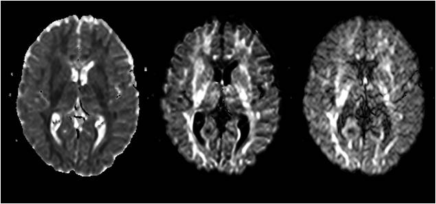
For mono-exponential model:

o ADC (T): Apparent Diffusion Coefficient (Trace) image. The generated ADC (T) map is scaled so that the pixels are in units of 10-5 mm2/s. For number of diffusion directions = 1, the ADC map represents the ADC along the applied gradient direction. For 3 diffusion directions, the ADC(T) map is generated from the geometric mean of the ADC in each of the three gradient directions. Applicable only to mono-exponential model.

o T2-corrected bMax: This map is similar to the bMax images (where bMax represents the maximum b-value), but with the T2-effect (also called 'T2-shine through') removed from the image. This is done by calculating the theoretical signal intensity of the bMax image according to the estimated ADC value.

o bMax: This is simply a copy of the bMax images from the input dataset and are only included for convenience (e.g. for direct comparison with T2-corrected bmax images). Applicable only to mono-exponential model.

o 'Anisotropy': Generates a pseudo anisotropy map based on the difference in ADC values in the three gradient directions (based on the standard deviation of the trace map). This option is only enabled for 3 diffusion gradient directions. Note that this image does not represent true anisotropy since at least six gradient directions are needed to determine anisotropy in three dimensions.

o Estimate DWI image for b-value…: estimates the DWI image for a given b-value. This is done by solving for fothe exponential expression for the scaling constant (A) with the estimated ADC and user-supplied b-value.

For bi-exponential and mixed model:

o ADC (fast): Parametric map of D_{fast} in the bi-exponential model.

o ADC (slow): Parametric map of D_{slow} in the bi-exponential model.

o Vol fraction (fast): Parametric map representing the volume fraction of the fast component, f_{fast}, in the bi-exponential model.

o Vol fraction (slow): Parametric map representing the volume fraction of the slow component of, f_{slow}, in the bi-exponential model.

When applying the mixed model option then only the D_fast map will contain non-zero values when a mono-exponential fit is found optimal for a given pixel.

Chi-square: Pearson’s cumulative test statistic for the chi-square test on the sum of squared errors from the least-squares fitting.

Sample output images from DWI module: ADC map (left) 'T2-corrected' b-max image (centre) and b-max image (right)