Theoretical background - Vessel Architectural Imaging

Vessel Architectural Imaging (VAI) is a new extension to conventional dynamic susceptibility contrast (DSC) MRI. In VAI-based perfusion imaging, one makes use of the known difference in microvascular sensitivity of the spin echo (SE) versus gradient echo (GRE) signal to MR contrast agents  [1]. In short, the SE signal has been shown to have peak contrast agent sensitivity to vessels in the micron range (capillaries), with falling sensitivity for larger vessels whereas the GRE signal has increasing contrast agent sensitivity up to large macrovessels. Hence, by acquiring both a SE and a GRE in a single DSC-MRI sequence, different properties of the microvasculature can be probed [2]. The VAI methodology builds on earlier work, especially by Kiselev et al, which termed the double echo SE/GRE approach ‘vessel size imaging’ (VSI) [3] – with the main difference that in VAI, a more systematic and parameterized analysis of the SE-GRE correlations are performed.

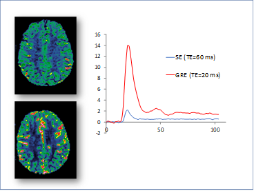
Figure 1: Examples of relative cerebral blood volume (CBV) maps obtained from respectively a SE-signal (top) and a GRE-signal (bottom) in a double echo SE-GRE echo planar imaging (EPI) acquisition.

Figure 1 shows examples of relative cerebral blood volume (CBV) maps obtained from respectively a SE-signal (top) and a GRE-signal (bottom) in a double echo SE-GRE echo planar imaging (EPI) acquisition. The more dominant presence of large vessels in the GRE-CBV map is evident. 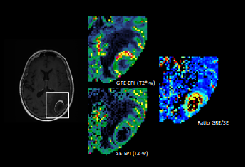The much smaller dose-response in the SE signal is also evident (blue curve vs red curve) – in spite of a longer TE in the SE readout (60 ms vs 20 ms), due to the generally lower sensitivity of SE to the contrast agent, as the long-range susceptibility effects (T2*-effects) are refocussed by the 180 degree refocussing pulse used to form the SE.

The difference in microvascular SE vs GRE response can be seen even more clearly in figure 2, in a patient with a brain metastasis. Again, we see CBV maps from GRE (middle top) and SE (middle bottom) and the ratio of the two in the are of the lesion (right image). The GRE-based CBV map clearly shows the presence of more large vessels in the tumor region compare to the SE-CBV map.

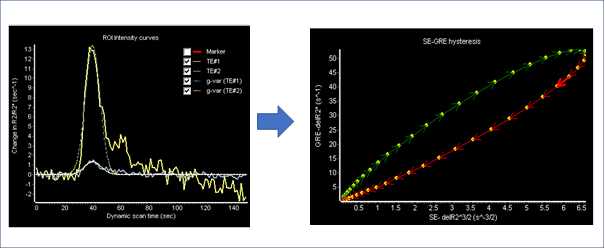
Figure 2: Example of the differece in microvascular SE vs GRE response.

In VAI based analysis, the pixel-wise GRE and SE dynamic signals are converted to change in R2 and R2*, respectively for the SE and GRE signals. The resulting deltaR2 values are then raised to the power of 3/2 and a gamma variate (or Gaussian) function is fitted to the resulting time curves. The fitted curves are plotted with delR2^3/2 along the x-axis and delR2* along the y-axis, forming the characteristic hysteresis loops. The hysteresis loops are characterized by the loop direction, long axis, slope of long axis and the area of the loop, properties shown to be related to microvascular properties [4]. In the VAI module, the voxel-wise loop direction is visualized by the arrows making up the loop as well as the arrow color (figure 3 b).

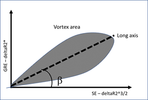
Figure 3: Characteristic hysteresis loop generated by plotting Gamma fitted SE vs GRE signals. Note that the direction of the loop is indicated by the color and direction of the arrows.

Following the convention or recent literature, the following metrics are extracted from the pixel-wise hysteresis curves (see figure 4):

. VAI vascular fraction (Vf) . Vf is defined as the long axis of the hysteresis loop (figure 3).

A. Vortex area (VA) . This is defined as the shaded region in figure 1 b. The cortex area can optionally be scaled by Vf so that VA(scaled) =VA/Vf. VA can also optionally be colored according to loop direction so that loops with clockwise loop directions have warm colors and negative loop directions have cold colors (figure 2).

B. Vortex direction . Binary image where a value of 1 equals clockwise loop direction and a value of -1 equals CCW direction.

C. Peak shift : The shift in the peak (fitted) SE vs GRE signals. Positive shifts for SE leading GRE signal.

D. Vessel calibre. Defined by the slope of the long axis (figure 3 b)

E. Vessel size image (VSI): Defined by  where is defined in figure 4, ADC is the apparent diffusion coefficient and CBV is normalized cerebral blood volume obtained from the GRE signal.

Note that in order to obtain (semi-) quantitative estimates of mean vessel size (f), the apparent diffusion coefficient, ADC, is required. This should be generated separately and included in the analysis, as explained in Diffusion weighted analysis.

Figure 4: Characteristic hysteresis loop generated by plotting Gamma fitted SE vs GRE signals .

Examples of different VAI-related perfusion maps are shown below (figure 5).

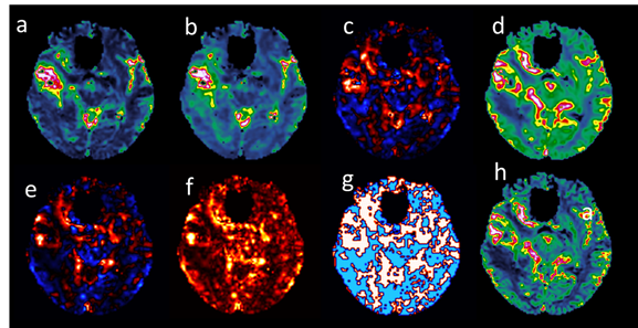
Figure 5: Sample VAI related perfusion maps: Vessel size index (a), Vessel calibre (b), peak shift (c), Vascular fraction (d), Vortex area (direction sensitive) (e), Vortex area (f), vortex direction (g) and for reference, normalized CBV (h).

Sequence requirements for VAI

In order to perform VAI analysis, a double echo EPI sequence is needed where the first echo is a GRE readout (typical TE 20-30 ms) and the second echo is a SE readout (typical TE 80-120 ms). The temporal resolution should be as high as possible (more important than for standard DSC-MRI) and sampling interval should preferably by 1.5 sec or less .  It should be noted that the SE and GRE parts cannot (currently) be acquired as two separate scans but need to be integrated in a single EPI acquisition. Based on the literature, VAI-compatible sequences are available as research options from most major vendors.

References:

[1] Weisskoff, R.M., Zuo, C.S., Boxerman, J.L. & Rosen, B.R. Microscopic susceptibility variation and transverse relaxation: theory and experiment. Magn. Reson. Med. 31, 601–610 (1994)

[2] Emblem et al. Nature Med; 19:9 (2013)

[3] Kiselev, V.G., Strecker, R., Ziyeh, S., Speck, O. & Hennig, J. Vessel size imaging in humans. Magn. Reson. Med. 53, 553–563 (2005)

[4] Digernes et al. J Cereb Blood Flow Metab. 2017 Jun;37(6):2237-2248