DCE
analysis options
More
options relating to the DCE analysis can be accessed from the <Options>
button at the bottom of the window.
The following menu
will appear:
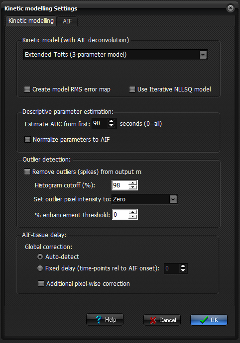
Kinetic modelling
Choose
between the following kinetic models (see 'Theory' section for more details):
- Extended Tofts (3-parameter model)
- Tofts-Kermode (2-parameter model)
- Patlak (2-parameter model)
- Two-compartment exchange (TCx)
(4-parameter model)
- Incremental model
The
incremental model will use the best adapted model at any point. You can also
choose to generate a model selection map, showing which model was most
optimal on a pixelwise basis. The following code is used: dark blue= Vp only (no leakage); light blue= Patlak; yellow =
Kermode (no Vp); green= Extended Tofts; red:
two-compartment exchange (TCx).
Use iterative NLLSQ model: By
default, the convolution integral forming the basis of DCE kinetic modelling
(see 'Theory' section) is solved by matrix inversion, by re-casting the
convolution integral to a matrix equation, yielding a fast and efficient
way of estimating the kinetic parameters (see Murase, K Magn Reson Med 51(4) 2004). The convolution integral can,
however, also be solved by standard iterative non-linear least squares
(NLLSQ) methods whereby the sum of squares error between the data and the
fitted function is iteratively minimized. Under certain conditions, the NLLSQ
approach may provide more correct parameter estimates, but at the cost of
much longer processing times. This option is therefore mainly suggested for
use in the 'interactive ROI mode' and not for parametric mapping.
Descriptive parameter estimation:
Use
this to set the time-range used for the AUC calculation. When Normalize parameters to AIF is
selected, the values of descriptive parameters like AUC, upslope and washout
are normalized to the corresponding values of the AIF.
Remove spikes in output maps: when this option is
checked, outlier values (spikes) are removed from the output maps. Such
spikes e.g. can occur due to unstable curve fitting
conditions with noisy input signal. You can further specify if outlier
pixels should be set to zero or to the maximum pixel value in the image
(after outliers have been removed). The Histogram cutoff value
specifies the percent cutoff for outlier
definition. if this value is set to e.g. 98% then
the upper 2% of the pixel values in the output data is treated as outliers.
% enhancement threshold: specifies
the minimum amount of enhancement (signal difference between baseline and
maximum value) required for a given pixel to be included in the
analysis. If set to 0% then all pixels (above general noise threshold, if
applied) are analyzed.
AIF-tissue delay:
The
kinetic models used for DCE-analysis inherently assume that the AIF and
tissue response contrast onset occur simultaneously. In practice, however,
there may be a significant delay between the AIF onset and the tissue onset,
and this delay me also vary between tissue types and between normal
tissue and pathology. nordicICE implements different strategies to
correct for possible AIF-tissue delays:
Auto-detect: when
selected, a global correction is applied to align the AIF with the global
(average time-intensity curve) for the entire image volume.
Fixed delay: when selected, the specified
fixed delay (in terms of number of image time-points) is used for the global
AIF-tissue delay correction
Additional pixel-wise correction: when
selected, additional pixel-wise delay correction is applied. Note that this
option will increase processing time.
AIF options
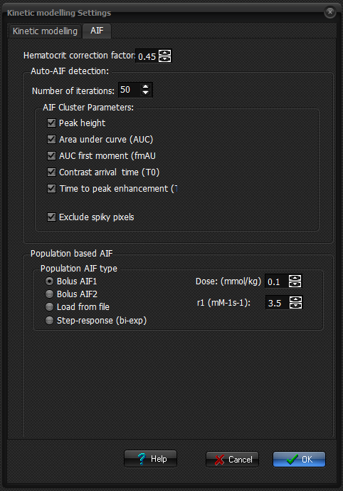
Hematocrit correction factor: Specifies
the factor used to estimate plasma concentration based on the whole blood
signal response. This value is typically set equal to the average hematocrit in the study population.
Auto-AIF detection
The
cluster technique used for automatic AIF detection can be optimized for
various parameter settings, which can be specified here.
Population based AIF
Two
different shaped population based AIFs are included.
When 'Population based AIF' is selected in the main menu of the DCE module,
the application will use the AIF specified here. A ‘population
based AIF’ as used here is a standard AIF derived from a
multi-compartment kinetic model of the expected shape of a contrast bolus in
the brain following a rapid injection in a ‘standard’ person. The
kinetic model used to obtain the standard AIF is described in van Osch MJ et al. Magn Reson
Med.2003 Sep; 50(3): 614-22. The two different pre-defined AIFs differ in
sharpness and maximum amplitude.
Additionally,
you can define your own AIF as a binary file and use this in the analysis. If
specifying your own AIF from a binary file, the number of entries in the file
must match the number of dynamic time-points in the raw data. You also need
to specify the temporal resolution of the supplied AIF. If different from
that of the dynamic data, the provided AIF will be re-sampled to match the
resolution of the imaging data. The amplitude values of the AIF entries are
assumed to reflect the concentration of the contrast agent at each time-point
(in units of mM ).
You
can also define a bi-exponential AIF where all parameters can be defined
manually.
For
all predefined AIFs as defined above, the relaxivity in blood (in units
ofmM-1s-1) of the contrast agent used need to be specified since the AIFs
here are represented in units of contrast agent concentration (mM )and need to be converted in the relaxation rates (1/R1
or 1/R2,R2*, depending on acquisition type). Default relaxivity values are provided
based on ‘standard’ gadolinium chelates at 3.0 T. For T2/T2* based
perfusion imaging, the actual in vivo blood relaxivity is more complex, and
some studies suggest a quadratic dose-response. An option of model a
quadratic dose-response (as described in vanOsch et
al Magn Reson Med 49(6): 1067-1076).
Related topics:
Kinetic modeling
theory
|