Kinetic Modelling Theory

Dynamic Contrast Enhanced (DCE) MRI analysis is the commonly used term to describe the analysis of the transient effect of a contrast agent (CA) on the measured signal intensity (or change in relaxation rate in the case of MRI) in the tissue of interest following a rapid bolus injection of the CA. The effect of the agent is analysed using an appropriate kinetic model, describing the time-dependent distribution of the CA in tissue. The contrast agents currently used in DCE analysis are most commonly small molecular weight agents (like Gd -DTPA and similar chelates), which are renally excreted with a half-life in blood limited by the glomerular filtration rate (GFR) of the kidneys. 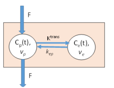The kinetics of these agents in tissue can generally be described by a so-called two-compartment exchange (TCx ) model (see e.g. Sourbron et al Magn Reson Med, 2009 and Tofts et al. JMRI 1999 for details) .

The two-compartment exchange model is illustrated in Figure1 below.

Figure 1. Two-compartment exchange (TCx ) model describing the capillary passage, and extravasation of contrast agent (CA) in tissue. The CA enters the capillary volume due to tissue blood flow, F, and is initially distributed in the tissue plasma volume, V_p , but is gradually equilibrated to the extravascular, extracellular space (EES), with volume fraction V_e at a rate determined by the rate constants K^trans and k_ep, where K^trans =k_ep ^. V_e .

Although nordicICE provides analysis with the full TCx model, this model has four independent model parameters (F, V_p, V_e, K^trans) and may give unstable results when applied to pixel-wise dynamic MRI data if SNR is too low (Sourbron and Buckley, Magn Reson Med, 2011), and different simplifications and assumptions are therefore commonly applied to obtain stable results, as described in more detail below.

The dynamic dose-response curve following a rapid injection of a CA in a two-compartment system is typically described by a wash-in phase (driven by tissue perfusion, F, and K^trans ) followed by a wash-out phase (driven by k_ep and plasma clearance). A typical curve is shown in Figure 2 also indicating some common descriptive metrics of the dynamic curve.

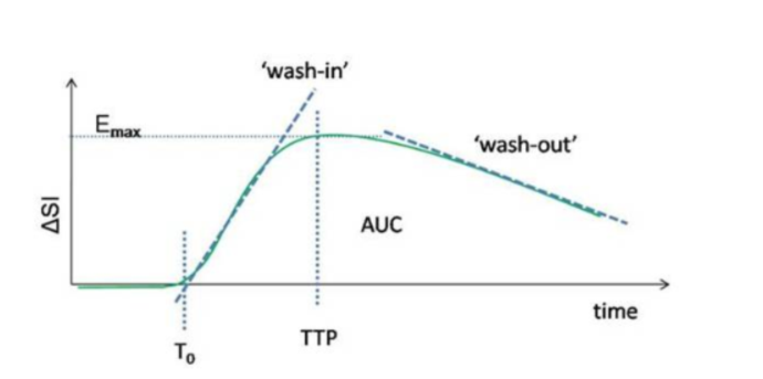
Figure 2. Typical dynamic dose-response following rapid contrast injection in a two-compartment exchange system, and corresponding curve parameters. AUC is the area under the dynamic response curve and TTP is the time to peak enhancement.

In case of very slow leakage, large EES or too short total sampling time, the wash-out phase can be ill defined. Also, the wash-in phase can often be bi-phasic with an initial steep slope (perfusion driven) followed by a reduced wash-in rate (K^trans driven).

The descriptive parameters described above do not directly reflect the underlying parameters of the kinetic model described in Figure 1. To extract these tissue specific kinetic parameters, the tissue response curve, and the arterial input function (AIF, describing the dynamic concentration time curve of the bolus passage in an artery feeding the tissue of interest) must be used as input to an appropriate mathematical model of the CA kinetics. As mentioned above, the full TCx model is complex, and simplifications are typically applied to obtain robust results when attempting to fit the pixel-wise dynamic data to the model.

The kinetic models available in nordicICE are summarized below.

1. Two-compartment exchange (TCx) model

This is the complete four-parameter model as shown in Figure 1, including both perfusion (F), plasma volume (V_p), K^trans and extracellular extravascular volume (V_e). The full model is mathematically complex, and the resulting impulse response is a bi-exponential function of the four model parameters. In nordicICE, the model is estimated by matrix inversion, as described in: Flouri et al Magn Reson Med (2016)

2.    Extended Tofts (ET) model.

This model assumes rapid flow (perfusion) relative to the sampling rate of the MRI sequence so that the CA transit time through tissue is essentially instantaneous. Under these conditions, it can be shown that the total CA in tissue is given by;

Eq 1

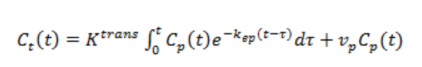
where C_p is the CA concentration in plasma and C_t is the total tissue CA concentration. Eq. 1 is also-called convolution integral, describing the CA kinetics (CA concentration change) in tissue following a bolus of CA initially present in the arterials feeding the tissue. In DCE-MRI, C_p (t) is determined from a well-defined artery (arterial input function, AIF) feeding the tissue of interest.

    3.    Tofts-Kermode (TK) model
This is a simplification of the ET model where the plasma volume is assumed to be negligible so that:

Eq 2 

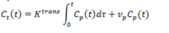
    4.    Patlak model
This model assumes the back-flux of CA from EES to plasma space to be negligible during the measurement time (i.e. exp ( -k_ep T ) ⁓ 1, where T=total measurement time). The kinetic model then becomes:

Eq 3

The advantage of the Patlak model is that is can be linearized, e.g. the expression can be re-cast in to a linear form so that K^trans and v_p can be determined by linear regression analysis (compared to non-linear regression for Eqs 1,2), which is generally more stable and less sensitive to image noise. The Patlak model can therefore be a good alternative if leakage rates are known to be low or when the DCE-MRI data has low SNR, giving poor curve fits for the non-linear models.

    5.    Incremental model

This method iterates through multiple models with increasing complexity and number of model parameters (Bagher-Ebadian et al, Magn Reson Med, 2012). For each tested model, the goodness-of-fit of the model to the data is compared to the fit of previous (less complex) model and a statistical test (F-test) is performed to test if the fit is significantly better than for the previous (less complex) model, justifying the increased complexity. The following models are included in the incremental testing:

a.      Noise only (zero V_p , K^trans and k_ep ) -> Pixels shown as black in model selection map

b.      No leakage (Non-zero V_p ;  zero K^trans and k_ep )  -> blue pixels

c.       Patlak model (non-zero K^trans and V_p , zero k_ep ) -> cyan pixels

d.      Tofts-Kermode model (non-zero K^trans and k_{ep ,} zero V_p ) -> yellow pixels

e.       Extended Tofts model (non-zero V_{p ,} K^trans and k_ep ) -> green pixels

f.        Two-compartment exchange (TCx) model (F, V_p, V_e and K^trans) -> red pixels

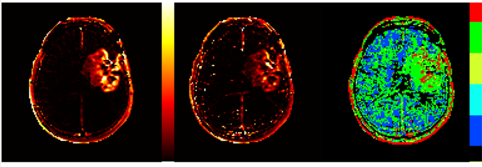
Figure 3 Sample K^trans parametric maps obtained with Two-compartment exchange (TCx) model and Patlak model. Note that use of Patlak model here provides less noise in the resulting map. Despite the Patlak based model map appearing less noisy, the model selection map (obtained by using the “incremental modelling” option) indicates that best fit in tumor region is obtained using either ET model (green) or TCx model (red) models. Note that in the model selection map palette has six distinct colors - one of each model to be tested, as described above.

Colour map for incremental model:

Kinetic modelling with vascular deconvolution

If the arterial input function (AIF) can be measured then the equation describing the selected kinetic model (Eqs . 1-3)   can be solved using standard numerical methods. In nordicICE, the AIF can be determined from many different methods, ranging from manual detection from user selected ROI, global automatic detection, or region specific automatic detection and finally using pre-defined (population) AIFs.     Figure 4 shows a sample AIF, tumor tissue curve and corresponding curve fit. The AIF contains signal from whole blood whereas the kinetic model assumes that we measure the plasma concentration of contrast agent. We therefore also need to scale the AIF signal according to the blood hematocrit (Hct ) since C_AIF = (1-Hct)C_p .The Hct can be specified in nordicICE but is by default set to 0.45.

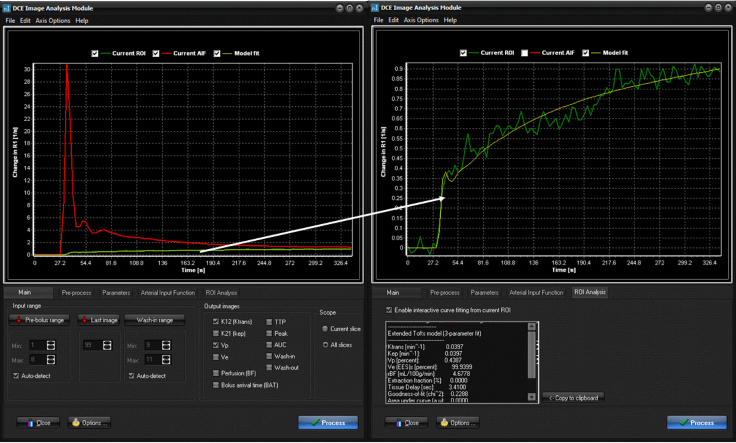
Figure 4. AIF determination and model fit visualization in nordicICE. Here, the AIF (red curve) was determined using the “automatic detection” option. The right panel shows the interactive curve fit option where the curve fit (yellow line) of a ROI in a tumor region (green curve) is shown, using the “ incremental model” selection option. The kinetic parameters obtained from the curve fit is shown in the panel below the curve.

Estimation of concentration time curves (CTC)

The kinetic models used to MRI-DCE analysis explicitly assumes that the CA concentration (C) is known. In MRI, the CA concentration cannot be measured directly and has to be derived from the observed change in MR signal intensity (SI) in response to the presence of the CA in tissue. One common assumption is that the change in 1/T1 relaxation rate is proportional to C, which is valid as long as there is a fast water exchange between water protons in tissue and the paramagnetic center of the CA. Given this assumption, C can be estimated (in relative units) given the change in 1/T1 relaxation rate can be measured. From strongly T1-weighted sequences, it is often assumed that the change 1/T1 is proportional to the change in SI. From this assumption, relative change in 1/T1 (and hence C) can then be estimated simply from the relative change in SI (either in absolute units or as a percent change). Both these conversion options are available in the DCE module and are typically used if the exact details of the MR sequence used are not known or a sequence is used where the signal response cannot be expressed in a simple analytical form (e.g. non steady-state sequences). The DCE module also enables exact estimation of change in 1/T1 for specific MR sequences. The two types of sequences which can currently be modelled are:

· Spoiled gradient echo (GRE) sequences. This is the most common sequence used in DCE imaging and is a class of sequences where the SI is given by the following expression:

Eq. 4

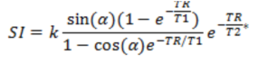
where k is an (unknown) constant, α is the flip angle, TR is the repetition time, T1 and T2* are the relaxation times and TE is the echo time.

· Saturation recovery (SR ) This is an alternative to the standard spoiled GRE sequence where the DCE signal is read out following given delay after a 90 degree preparation pulse. Here, the SI is given by :

Eq. 5

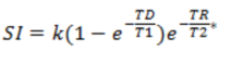
where TD is the delay time (time from 90-degree pulse to start of acquisition). This class of sequence has been shown to be less sensitive to water exchange effects when short TD-times are used (Larsson et al. Magn Reson Med, 2001).

By assuming the TE<<T2*, the change in 1/T1 can then be determined if TR and flip angle (GRE) or TD (SR)are known, in addition to 1/T1 at baseline (1/T10). In the DCE module 1/T10 can either be set at a fixed values (1000 ms as default) or can be taken from a T1-relaxation map estimated separately (either using the nordicICE T1-relaxation module or by separate software) . For MR sequences which cannot be modelled by any of the two expressions, the relative change in 1/T1 must be estimated from the relative (or absolute) change in SI, which then assumes that this SI is linearly related to 1/T1 changes induced by the CA in tissue and blood.