T₂ / R₂ relaxation analysis

Main Menu: Modules -> T2 Relaxation analysis

Generates an image where the pixel intensities represent transverse relaxation times or rates; T2/ T2* (in ms) or R2/R2* (in 1/sec) values. The image is calculated based on a multi-echo (two or more) series, either from a spin-echo (T2/R2) or gradient echo (T2*/R2*) echo train. The transverse relaxation times are calculated by fitting the multi-echo signal intensity data to the following function:

SI = A exp(-TE • R2) + C where A and C are constants, SI is the signal intensity at a given echo time TE and R2 is the transverse relaxation rate ( 1/T2 or 1/T2*). The C variable is set to zero if the <apply baseline correction> option is not enabled (see below).

Note: for multi-slice input data, the image selection tab must be set to <All> in order to generate relaxation maps for all slices.

The following options are available:

T2 Relaxation analysis settings

Parameters

Here you set the input parameters relevant for the curve fitting:.

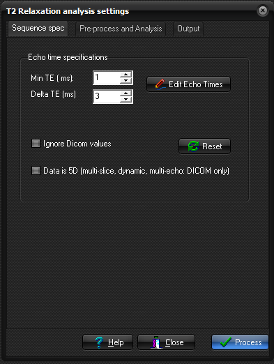
Echo time specifications: 

Selected if a constant echo spacing is used. Minimum TE is the TE of the first echo and delta TE is the echo spacing of consequitive echoes after the first echo. All TE values are in msec.

Edit Echo Times: 

The TE values are specified in a list. This would be used in situations where the echoes are sampled at uneven intervals.

Ignore Dicom values: 

Check this box if TE values are found in the DICOM header, but one wishes to use other values.

Data is 5D (multi-slice, dynamic multi-echo): 

This can be used to create a dynamic T2-map. Requires that data has several echos acquired per dynamic time point.

 

Pre-process and Analysis:

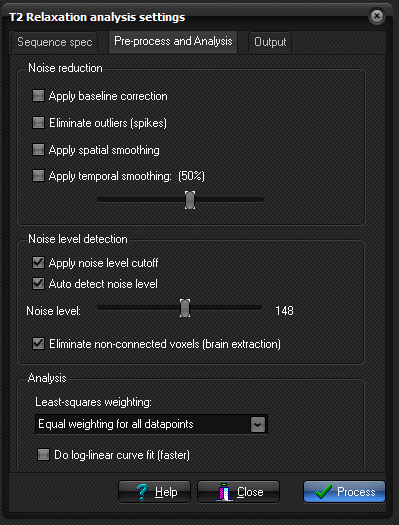
Apply baseline correction: 

An additional fitting variable (C) is used to account for non-zero baseline signal level. The offset value is only included in the curve fit if the signal reaches a signal level at high TE values close to the noise level.

Eliminate spikes:

Remove very high values from the output map.

Apply spatial smoothing:

Apply a nearest neighbour smoothing kernel to the raw data prior to curve fitting.

Apply temporal smoothing:

The dynamic time signal is smooted (low-pass filtered), to reduce effects of noise and spikes in the dynamic signal response. This smoothing does not affect spatial resolution but may reduce the ability to detect rapid signal changes. If temporal smoothing is selected the degree of smoothing can be varied using the slider.

Noise Threshold

Auto Detect: Automatically determine the noise level in the input images (default). The noise level can be modified using the slider.
Show noise level cutoff: Show the selected noise threshold as red pixels in the input images. All pixels colored red are excluded from the analysis.

 

Analysis:

It is possible to use different weigthing for the different datapoints. Variable weighting can be useful in order to apply less weight during the curve fitting procedure to data points known to be affected by noise - or to ensure good curve fit for specific parts of the curve. Or alternatively, very high amplitude data points can be given reduced weighting to obtain better fits for data close to zero values.

Output

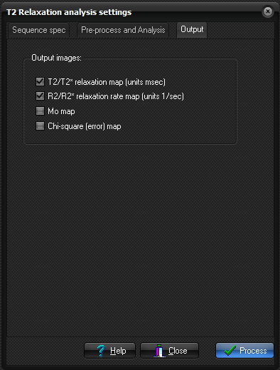
Output Image types: 

• Rr/R2* relaxation rate map: pixel values represent inverse relaxation times (1/T1) in units of 1/sec.
• T2/T2* relaxation rate map: pixels values represent relaxation times in units of msec. 
• M0 map: This map represents the relative equilibrium magnetization obtained from the curve fit.
• Chi-square map: An additional output image is generated which represents the pixel-wise  'goodness of fit' (described by the chi-square parameter resulting from the least squares fit) 

Related topics: