Starting
the perfusion module
The perfusion module main window will appear together with two
image windows - one containing the original input data and one new window constaining the converted time series for the current
slice. The main perfusion window contains multiple tabs (task groups),
as described below as well as a graph showing the dynamic signal response (mean
curve) for the current slice.
Perfusion
module interface
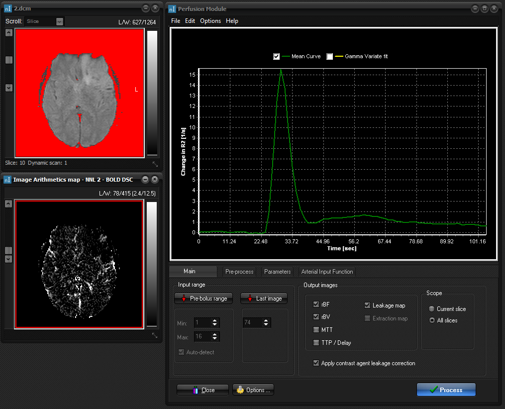
Initial screen layout when starting the perfusion module with a
T2*-weighted dynamic multi-slice MR data set (top image window). The default
curve shows the global (average) signal curve for the dynamic series for
the current slice after signal conversion to change in R2*. Note that
the displayed time curve should have a positive peak amplitude and a zero
(approximate) bassline value. The signal conversion type is set under the
<Parameters> tab. The second image window contains the dynamic image
series for the selected slice after signal conversion. If the slice is
changed in the main image window, the dynamic image window is updated to
reflect the new slice. By default, the noise threshold level is shown as red
overlay in the input dataset. All pixels in red indicate pixels excluded from
further perfusion analysis. By default, the noise level is estimated
automatically, but can be adjusted by the user under the
<Pre-process> tab.
Note that ROIs can be drawn in the converted dynamic time series
window using any of the ROI shapes. When a ROI is drawn, the dynamic curve
for the selected ROI will be displayed instead of the average curve for the
entire image.
The Perfusion Module menu is sub-divided into four groups
(tabs):
1. Main
2. Pre-process
3. Parameters
4. Arterial Input
Function
The Arterial Input Function tab is not used if vascular
deconvolution (correction for AIF) is not applied.
Gamma variate fitting
You can specify the dynamic data to be fitted to a gamma
variate function, by turning on the Gamma variate fit on the top of the
graph. This is an asymmetric derivation of a Gaussian curve describing the
theoretical concentration-time curve of a first-pass bolus through tissue
(see e.g. Bjornerud et al Magn Reson Med 47:298:304
(2002) for details). By default, the perfusion analysis is performed on the
raw (unprocessed) first-pass curve within the limits set by the pre-bolus
range and image range. This is the quickest method to obtain
relative perfusion maps since no curve fitting is involved. However, analyzing the raw first-pass curve may give rise to some
spurious variations in the perfusion values due to recirculation effects and
general effects of noise. Fitting to a gamma variate function to the
fist-pass curve can produce smoother maps if the input data is noisy and will
also reduce the effect of contrast agent recirculation. The drawback of
fitting the first-pass data is that the data may not fit the model function
well - in areas of abnormal perfusion. Also, gamma variate fitting can
itself be unstable if data is noisy.
When gamma variate fitting is selected, an additional output map
called a chi-square map can be generated. This image represents the
'goodness of fit' of the raw data to the gamma variate model function for
each pixel. To generate this map, turn it on in the Options - Output menu.
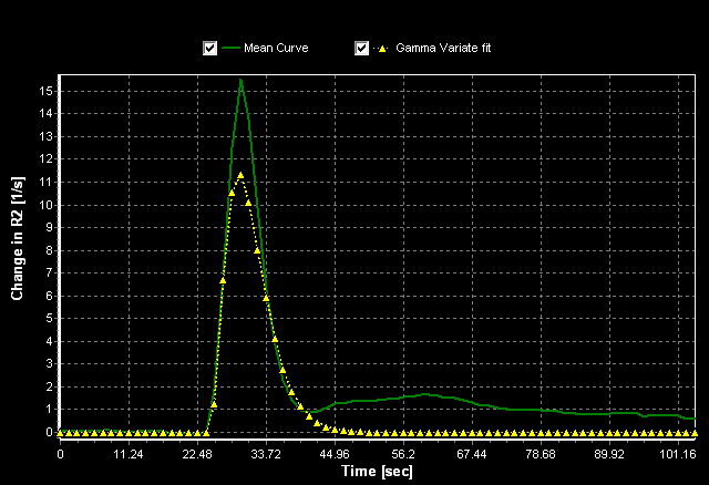
When gamma variate fitting is selected, the dynamic curve will
interactively be fitted to a gamma variate function (shown in yellow) as seen
below.
Note that if gamma variate fitting is combined with AIF
deconvolution, then the AIF will be fitted to a gamma function also.
Next step:
Main settings

|